从理论到代码：逐步实现和分解GPT-2模型的代码。

这篇文章是第二部分，请先阅读这里的GPT模型演变，以更好地理解我们为什么选择GPT 2模型。

在这篇文章中，我们将讨论GPT-2模型的实现，探索其架构以及如何支持最先进的语言生成技术。通过逐步编写GPT-2模型，我们将揭示其变压器模块、注意力机制和前馈网络的内部工作原理，同时理解为什么这种架构在生成连贯和语境丰富的文本方面表现出色。无论您对神经网络已经很熟悉还是对变压器还很陌生，这篇指南都将带您在构建和微调GPT-2时获得实用的视角。

我们将首先将GPT-2模型分解为其主要组成部分，然后逐步实现每个模块。

GPT-2模型解析:

• 令牌嵌入
• 位置编码
• Transformer Blocks- Multi-Head Attention- Layer Normalization- Feed-Forward Neural Network- Residual Connections Transformer块- 多头注意力- 层归一化- 前馈神经网络- 残差连接
• 输出层

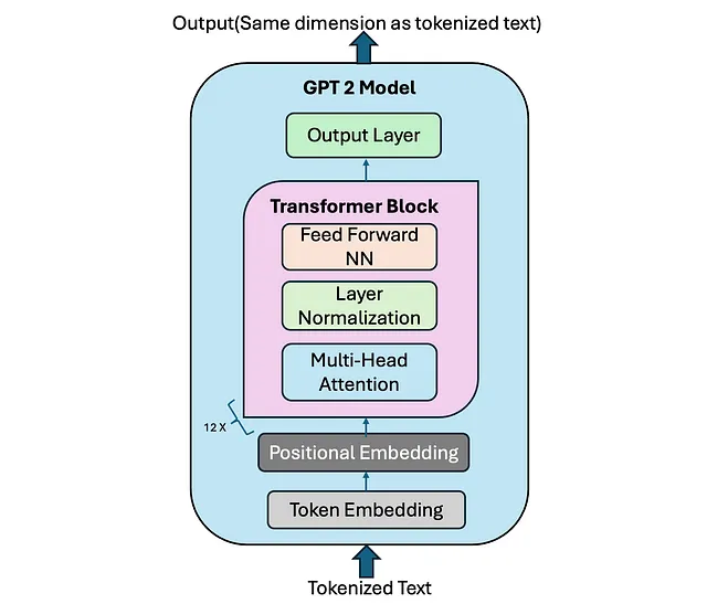
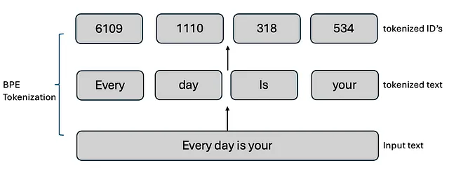
在我们讨论和开始编码每个组件之前，我们看到输入到GPT-2模型的是标记化文本。最初，GPT-2模型使用字节对编码标记化，也称为BPE标记化。有关BPE标记化的更多信息可以在这里了解。

# 0 tokenize text
from transformers import GPT2Tokenizer

# Initialize the BPE tokenizer
tokenizer = GPT2Tokenizer.from_pretrained("gpt2")
text = "Every day is your"
encoded_input = tokenizer.encode(text, return_tensors='pt')  # Returns a tensor
print(f"Encoded input: {encoded_input}")

令牌化文本被送入GPT模型。让我们详细讨论一下GPT-2模型。我们导入我们需要的软件包，并设置一些配置变量，这些变量将在GPT-2模型（124M）中使用。

import torch
import torch.nn as nn
import math

# Configuration for GPT-2 124M
GPT_CONFIG_124M = {
    "vocab_size": 50257,    # Vocabulary size
    "context_length": 1024, # Context length
    "emb_dim": 768,         # Embedding dimension
    "n_heads": 12,          # Number of attention heads
    "n_layers": 12,         # Number of layers
    "drop_rate": 0.1,       # Dropout rate
    "qkv_bias": False       # Query-Key-Value bias
}

以下是模型中使用的关键变量的详细说明:

• vocab_size：定义词汇量大小，在我们的案例中为50,257个令牌，由BPE分词器确定。
• 上下文长度：代表模型的最大输入标记长度，受位置嵌入的限制。
• emb_dim：指的是标记输入的嵌入大小，其中每个输入标记被转换为一个768维向量。
• n_heads: 指定多头注意力机制中的注意力头数。
• n_layers: 表示模型中的Transformer块的数量，将在接下来的章节中实现。
• dropout_rate：决定放弃机制的强度，值为0.1表示在训练过程中有10％的隐藏单元会被放弃，以减少过度拟合。
• qkv_bias: 控制在计算查询（Q）、键（K）和值（V）张量时，在多头注意力机制的线性层中是否添加偏置向量。我们默认情况下禁用此功能，遵循现代大型语言模型中的常见实践。

令牌嵌入（点击此处了解更多）

Token embeddings负责将输入的标记（通常是单词或子词）转换为连续的数值向量，以便模型可以处理。这些嵌入可以捕捉标记的语义含义，并是模型表示和理解语言的关键第一步。

# 1. Embedding Layer
class Embedding(nn.Module):
    def __init__(self, vocab_size, embed_size):
        super().__init__()
        # Initialize the embedding layer with the specified vocabulary size and embedding dimension
        self.embed = nn.Embedding(vocab_size, embed_size)
    
    def forward(self, x):
        # Forward pass: convert input token IDs to their corresponding embeddings
        return self.embed(x)

# Test Embedding
# Create an instance of the Embedding layer using the configuration values
embedding = Embedding(GPT_CONFIG_124M["vocab_size"], GPT_CONFIG_124M["emb_dim"])
# Generate random input token IDs with shape (batch_size, seq_length)
input_ids = torch.randint(0, GPT_CONFIG_124M["vocab_size"], (2, 10))
# Apply the embedding layer to the input token IDs
embed_output = embedding(input_ids)
# Print the shape of the output embeddings
print(f"Embedding output shape: {embed_output.shape}")
# Assert that the output shape matches the expected shape
# Expected shape: (batch_size, seq_length, embed_size)
assert embed_output.shape == (2, 10, GPT_CONFIG_124M["emb_dim"]), "Embedding shape mismatch"

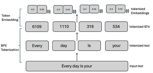
GPT-2使用嵌入层将每个标记（离散整数索引）转换为连续值的稠密向量，称为标记嵌入。这些嵌入是高维的，其大小由模型的隐藏维度定义（例如，对于GPT-2 small，隐藏维度为768）。

位置编码 (在这里了解更多)

在GPT-2模型中，使用位置编码来为模型提供关于序列中令牌顺序的信息，因为模型本身没有内建的方法来理解令牌的位置。不同于循环神经网络（RNNs）等模型，这些模型固有地按顺序处理数据，变换器架构可以同时处理所有令牌。因此，需要明确的关于令牌位置的信息来保留单词顺序的概念。

1. 在变压器中的位置编码：变压器架构，包括GPT-2在内，使用位置编码将关于序列中每个令牌位置的信息注入到输入嵌入中。这是通过给每个令牌的词嵌入添加一个固定的位置编码向量来实现的。
2. 正弦编码：GPT-2使用正弦位置编码，这是在原始Transformer论文中首次引入的（Vaswani等，2017年）。位置编码是基于令牌的位置pos和编码向量的维度i计算的。

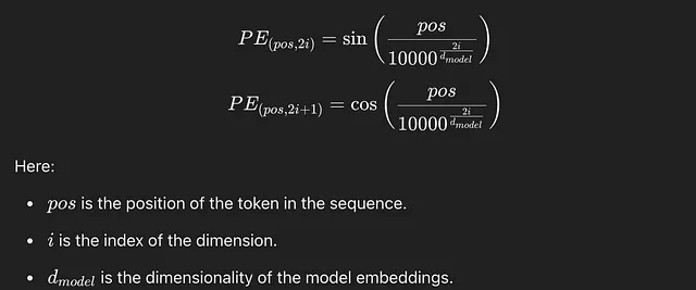
为什么选择正弦函数？：正弦函数之所以被选择，是因为它们使模型能够泛化到比训练中看到的序列长度更长的情况。正弦和余弦函数的周期性使模型能够学习不同位置之间的关系。此外，这些函数的平滑连续性赋予模型一些几何结构，用于识别位置模式。

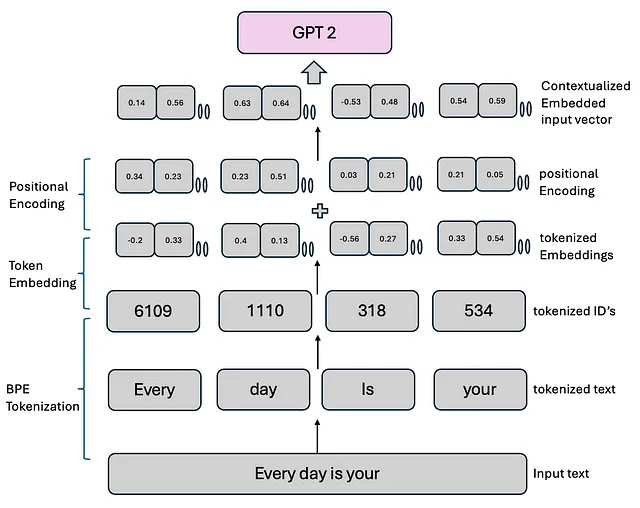
在GPT-2中，计算位置编码后，将其加到令牌嵌入中（在之前的步骤中生成），然后再馈送到变压器层。这使模型能够理解令牌位置，更好地捕捉序列关系，比如句子结构、排序和依赖关系。

# 2. Positional Encoding
class PositionalEncoding(nn.Module):
    def __init__(self, embed_size, max_seq_length=512):
        super().__init__()
        # Initialize a tensor to hold the positional encodings
        pe = torch.zeros(max_seq_length, embed_size)
        
        # Create a tensor for positions (0 to max_seq_length)
        position = torch.arange(0, max_seq_length, dtype=torch.float).unsqueeze(1)
        
        # Calculate the division term for the sine and cosine functions
        div_term = torch.exp(torch.arange(0, embed_size, 2).float() * -(math.log(10000.0) / embed_size))
        
        # Apply sine to even indices and cosine to odd indices
        pe[:, 0::2] = torch.sin(position * div_term)  # Sine for even indices
        pe[:, 1::2] = torch.cos(position * div_term)  # Cosine for odd indices
        
        # Register the positional encodings as a buffer (not a model parameter)
        self.register_buffer('pe', pe.unsqueeze(0))  # Shape: (1, max_seq_length, embed_size)
    def forward(self, x):
        # Add the positional encodings to the input embeddings
        return x + self.pe[:, :x.size(1)]

# Test Positional Encoding
# Create an instance of the PositionalEncoding layer using the configuration values
pos_encoding = PositionalEncoding(GPT_CONFIG_124M["emb_dim"], GPT_CONFIG_124M["context_length"])
# Apply the positional encoding to the output of the embedding layer
pos_output = pos_encoding(embed_output)
# Print the shape of the output after adding positional encodings
print(f"Positional Encoding output shape: {pos_output.shape}")
# Assert that the output shape matches the expected shape
assert pos_output.shape == embed_output.shape, "Positional Encoding shape mismatch"

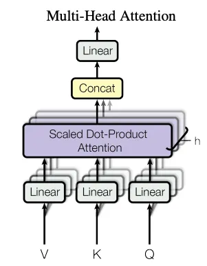
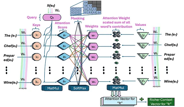
多头注意力 (在此处详细学习)

在上一篇关于注意力的文章中，我详细讨论了多头注意力。在高层次上，多头注意力机制分解为几个注意力头，每个头都专注于输入序列的不同方面。GPT-2不使用单一的注意力机制，而是并行地使用多个注意力头来捕获数据的更丰富的表示。

GPT-2 被设计为一次生成一个令牌的文本，其中每个令牌仅依赖于其之前出现的令牌。这被称为自回归建模，其中模型根据所有先前的令牌来预测序列中的下一个令牌。为了强制执行这一点，GPT-2 使用了掩码注意力，防止模型在训练期间查看未来的令牌以“作弊”。

# 3. Multi-Head Attention (Comments not added as explained in other article)
class MultiHeadAttention(nn.Module):
    def __init__(self, embed_size, num_heads, qkv_bias=False):
        super().__init__()
        self.embed_size = embed_size
        self.num_heads = num_heads
        self.head_dim = embed_size // num_heads
        
        self.query = nn.Linear(embed_size, embed_size, bias=qkv_bias)
        self.key = nn.Linear(embed_size, embed_size, bias=qkv_bias)
        self.value = nn.Linear(embed_size, embed_size, bias=qkv_bias)
        self.out = nn.Linear(embed_size, embed_size)
        
    def forward(self, x, mask=None):
        batch_size = x.shape[0]
        
        q = self.query(x).view(batch_size, -1, self.num_heads, self.head_dim).transpose(1, 2)
        k = self.key(x).view(batch_size, -1, self.num_heads, self.head_dim).transpose(1, 2)
        v = self.value(x).view(batch_size, -1, self.num_heads, self.head_dim).transpose(1, 2)
        
        attention = torch.matmul(q, k.transpose(-1, -2)) / math.sqrt(self.head_dim)
        if mask is not None:
            attention = attention.masked_fill(mask == 0, float('-inf'))
        attention = torch.softmax(attention, dim=-1)
        
        out = torch.matmul(attention, v)
        out = out.transpose(1, 2).contiguous().view(batch_size, -1, self.embed_size)
        return self.out(out

# Test Multi-Head Attention
mha = MultiHeadAttention(GPT_CONFIG_124M["emb_dim"], GPT_CONFIG_124M["n_heads"])
mha_output = mha(pos_output)
print(f"Multi-Head Attention output shape: {mha_output.shape}")
assert mha_output.shape == pos_output.shape, "Multi-Head Attention shape mismatch"

层归一化

层归一化在稳定和改进GPT-2模型训练中起着关键作用。它确保模型通过对每一层的输入进行归一化，能更有效地处理大规模数据，有助于防止梯度消失或梯度爆炸等问题，并在训练过程中改善收敛性。

层归一化通过将每个变压器层的隐藏单元激活标准化，确保它们具有零均值和单位方差，从而稳定了输入。它应用在自注意力和前馈层之前（在我们为变压器块编码时会看到），以确保模型训练效率高，并防止梯度爆炸或消失等问题。归一化过程有助于改善泛化能力，使模型对数据的内部变化不那么敏感，并使其能够有效处理大规模文本数据。

# 4. Layer Normalization (Just for explanation, we used nn.LayerNorm later)
class LayerNorm(nn.Module):
    def __init__(self, emb_dim, eps=1e-5):
        super().__init__()
        self.eps = eps
        self.scale = nn.Parameter(torch.ones(emb_dim))
        self.shift = nn.Parameter(torch.zeros(emb_dim))
    def forward(self, x):
        # Calculate mean and variance
        mean = x.mean(dim=-1, keepdim=True)
        var = x.var(dim=-1, keepdim=True, unbiased=False)
        
        # Normalize the input
        norm_x = (x - mean) / torch.sqrt(var + self.eps)
        
        # Scale and shift
        return self.scale * norm_x + self.shift

层归一化与批归一化- 批归一化是神经网络中广泛使用的归一化技术，让我们讨论一下它与层归一化的不同之处。批归一化在批维度上对数据进行归一化，而层归一化在特征维度上进行归一化。大型语言模型（LLM）通常需要大量的计算资源，硬件可用性或特定用例等因素可能会影响训练或推理过程中的批大小。层归一化通过独立于批大小对每个输入进行归一化，提供了更大的灵活性和稳定性，这对于分布式训练或在资源受限环境中部署特别有优势。

前馈神经网络

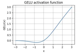
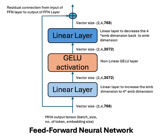
前馈网络（FFN）是变压器架构的一个关键组件，它在多头注意力机制的输出上操作。该网络用于进一步处理注意力输出并捕捉更复杂的转换。GPT-2在其前馈层中使用了GELU（高斯误差线性单元）激活函数，这是其设计的一个重要方面。

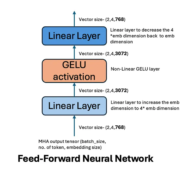
在GPT-2中，每个变换器块都包含一个前馈网络，由两个全连接层组成，它们之间应用了一个非线性激活函数（GELU）。

• 第一个线性层：来自多头注意力机制的输入通过一个全连接（线性）层传递。这个层扩展了输入的维度。
• GELU激活：在第一次线性变换之后，GPT-2应用GELU激活函数，引入非线性到模型中。GELU激活逼近正值x的恒等函数并顺利压制负值，比传统的ReLU等激活函数更有效地用于某些任务。它通过基于输入值的概率门控机制，允许对输入作出更细致的响应。



• 第二个线性层：经过GELU激活函数处理后的输出，然后通过第二个全连接层传递，将隐藏表示投影回模型的原始维度。

# 5. Feed-Forward Network
class FeedForward(nn.Module):
    def __init__(self, embed_size, ff_hidden_size):
        super().__init__()
        # First linear layer that transforms input from embedding size to hidden size
        self.fc1 = nn.Linear(embed_size, ff_hidden_size)
        # Second linear layer that transforms from hidden size back to embedding size
        self.fc2 = nn.Linear(ff_hidden_size, embed_size)
        # GELU activation function
        self.gelu = nn.GELU()
    def forward(self, x):
        # Forward pass: apply the first linear layer, then GELU activation, and finally the second linear layer
        return self.fc2(self.gelu(self.fc1(x)))


# Test Feed-Forward Network
# Define the hidden size for the feed-forward network (4 times the embedding size)
ff_hidden_size = GPT_CONFIG_124M["emb_dim"] * 4
# Create an instance of the FeedForward network
ff = FeedForward(GPT_CONFIG_124M["emb_dim"], ff_hidden_size)
# Apply the FeedForward network to the output of the multi-head attention layer
ff_output = ff(mha_output)
# Print the shape of the output after applying the FeedForward network
print(f"Feed-Forward output shape: {ff_output.shape}")
# Assert that the output shape matches the expected shape
assert ff_output.shape == mha_output.shape, "Feed-Forward shape mismatch"

残差连接-

残差连接在多头注意力和前馈网络层周围使用。这些连接将层的输入添加回其输出，创建一个用于梯度反向传播的快捷方式。残差连接通过使梯度更直接地通过网络流动，特别是在像GPT-2这样的深度模型中，防止梯度消失或爆炸。它们使更深的网络成为可能，没有残差连接，深度网络经常难以有效收敛。

数学上，对于每个子层（MHA或FFN），残差连接为：输出=层（x）+ x

残差连接保留原始输入，同时允许模型在其基础上学习额外的表示。

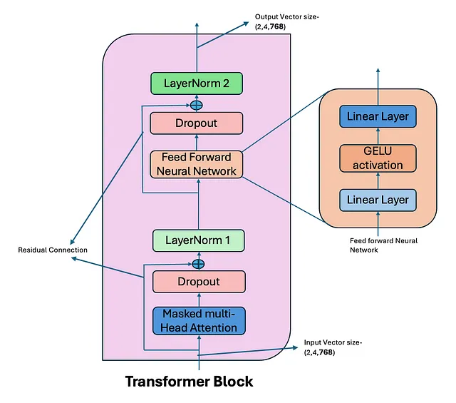
变压器模块

在GPT-2模型中，一个变压器块通过一系列步骤处理输入文本，它应用了掩码多头自注意力，其中每个标记关注序列中的先前标记来捕捉依赖关系。这个输出经过一个前馈网络（FFN）传递，用于转换数据以捕捉更复杂的模式。两个阶段都跟随着残差连接和层归一化，以确保稳定性和有效学习。

# 6. Transformer Block
class TransformerBlock(nn.Module):
    def __init__(self, embed_size, num_heads, ff_hidden_size, dropout=0.1, qkv_bias=False):
        super().__init__()
        # Initialize the multi-head attention layer
        self.mha = MultiHeadAttention(embed_size, num_heads, qkv_bias)
        # Initialize the feed-forward network
        self.ff = FeedForward(embed_size, ff_hidden_size)
        # Initialize layer normalization for the attention output
        self.ln1 = nn.LayerNorm(embed_size)
        # Initialize layer normalization for the feed-forward output
        self.ln2 = nn.LayerNorm(embed_size)
        # Initialize dropout layer
        self.dropout = nn.Dropout(dropout)
    def forward(self, x, mask=None):
        # Apply multi-head attention and add the residual connection, followed by layer normalization
        attention_output = self.ln1(x + self.dropout(self.mha(x, mask)))
        # Apply feed-forward network and add the residual connection, followed by layer normalization
        ff_output = self.ln2(attention_output + self.dropout(self.ff(attention_output)))
        return ff_output


# Test Transformer Block
# Create an instance of the TransformerBlock using the configuration values
transformer = TransformerBlock(GPT_CONFIG_124M["emb_dim"], GPT_CONFIG_124M["n_heads"], ff_hidden_size)
# Apply the transformer block to the output of the positional encoding layer
transformer_output = transformer(pos_output)
# Print the shape of the output after applying the transformer block
print(f"Transformer Block output shape: {transformer_output.shape}")
# Assert that the output shape matches the expected shape
assert transformer_output.shape == pos_output.shape, "Transformer Block shape mismatch"

通过变压器块的数据流程：

输入标记被嵌入到连续向量中，作为变形器块的初始输入。

1. 遮蔽式多头注意力：令牌嵌入通过遮蔽式多头自注意力机制传递，允许每个令牌注意先前的令牌，同时保持自回归建模约束。在此添加注意力丢失以提升泛化能力。
2. 残差连接和层归一化：注意力输出通过残差连接与原始输入结合，然后经过层归一化。
3. 前馈网络（FFN）: 标准化输出通过前馈网络传递，使用GELU激活进行非线性转换。在这里添加了FFN dropout以提高泛化能力。
4. 第二个残差连接和层归一化：应用另一个残差连接，然后是层归一化，确保下一个变压器块的稳定输入。

注意力失效和FFN（前馈网络）失效是用于防止过拟合并在训练过程中提高模型泛化能力的正则化技术。

以下是我们展开了前向方法，使其与上面的图像对齐。

# Forward function of Transformer block with more details 
def forward(self, x, mask=None):
    # Step 1: Apply Multi-Head Attention
    # The multi-head attention layer processes the input 'x' and returns the attention output.
    # The 'mask' is used to prevent attending to certain positions (e.g., for padding or future tokens).
    attention_output = self.mha(x, mask)  # Shape: (batch_size, seq_length, embed_size)
    # Step 2: Apply Dropout
    # Apply dropout to the attention output to prevent overfitting during training.
    attention_output = self.dropout(attention_output)
    # Step 3: Add Residual Connection
    # Add the original input 'x' to the attention output. This is known as a residual connection,
    # which helps in training deeper networks by allowing gradients to flow more easily.
    attention_output = x + attention_output  # Shape: (batch_size, seq_length, embed_size)
    # Step 4: Apply Layer Normalization
    # Normalize the output of the attention block to stabilize the learning process.
    attention_output = self.ln1(attention_output)  # Shape: (batch_size, seq_length, embed_size)
    # Step 5: Apply Feed-Forward Network
    # Pass the normalized attention output through the feed-forward network.
    ff_output = self.ff(attention_output)  # Shape: (batch_size, seq_length, embed_size)
    # Step 6: Apply Dropout to Feed-Forward Output
    # Apply dropout to the output of the feed-forward network.
    ff_output = self.dropout(ff_output)
    # Step 7: Add Residual Connection for Feed-Forward Output
    # Add the normalized attention output to the feed-forward output.
    # This is another residual connection.
    ff_output = attention_output + ff_output  # Shape: (batch_size, seq_length, embed_size)
    # Step 8: Apply Layer Normalization to Feed-Forward Output
    # Normalize the final output of the transformer block.
    ff_output = self.ln2(ff_output)  # Shape: (batch_size, seq_length, embed_size)
    # Step 9: Return the final output
    return ff_output  # Shape: (batch_size, seq_length, embed_size)

在GPT-2中，多个transformer块堆叠在一起（例如，GPT-2 small有12层，GPT-2 large有24层）。每个transformer块的输出作为下一个块的输入，逐渐完善令牌的表示。这种深度使得GPT-2能够捕捉文本中的长程依赖关系，从而提高其强大的语言建模能力。

输出层和GPT模型代码

在GPT-2中，最终的输出层负责生成序列中下一个符号的预测。一旦输入通过堆叠的变换器块，模型使用最终的输出来预测最有可能的下一个单词。以下是这个过程的工作方式：

fc_out层是一个全连接层。在输入令牌经过所有堆叠的变压器块之后，我们得到了一组经过优化的隐藏表示，对应于输入序列中的每个令牌。fc_out层将来自最终变压器块的每个令牌的隐藏状态，映射到词汇表的大小。这种映射产生逻辑值，表示模型对词汇表中每个可能令牌的信心程度。

这些逻辑值然后可以通过softmax函数传递，将它们转换为概率分布，从而使模型能够根据词汇表中每个标记被分配的概率来预测序列中最可能的下一个标记。

# 7. GPT-2 Model
class GPT2(nn.Module):
    def __init__(self, config):
        super().__init__()
        # Initialize the embedding layer to convert token IDs to embeddings
        self.embedding = Embedding(config["vocab_size"], config["emb_dim"])
        
        # Initialize positional encoding to add positional information to embeddings
        self.positional_encoding = PositionalEncoding(config["emb_dim"], config["context_length"])
        
        # Create a list of transformer blocks
        self.transformer_blocks = nn.ModuleList([
            # Each transformer block consists of multi-head attention and feed-forward layers
            TransformerBlock(config["emb_dim"], config["n_heads"], config["emb_dim"] * 4, config["drop_rate"], config["qkv_bias"])
            for _ in range(config["n_layers"])  # Repeat for the number of layers specified in the config
        ])
        
        # Final linear layer to project the output back to the vocabulary size for logits
        self.fc_out = nn.Linear(config["emb_dim"], config["vocab_size"])
        
        # Dropout layer for regularization
        self.dropout = nn.Dropout(config["drop_rate"])
    def forward(self, x, mask=None):
        # Step 1: Convert input token IDs to embeddings and add positional encodings
        x = self.dropout(self.positional_encoding(self.embedding(x)))
        
        # Step 2: Pass the embeddings through each transformer block
        for block in self.transformer_blocks:
            x = block(x, mask)  # Apply the transformer block with optional masking
        
        # Step 3: Project the final output to the vocabulary size
        return self.fc_out(x)  # Shape: (batch_size, seq_length, vocab_size)

# Test GPT-2 Model
# Create an instance of the GPT-2 model using the configuration values
model = GPT2(GPT_CONFIG_124M)
# Generate random input token IDs with shape (batch_size, seq_length)
input_ids = torch.randint(0, GPT_CONFIG_124M["vocab_size"], (2, 64))
# Apply the model to the input token IDs
output = model(input_ids)
# Print the shape of the output from the model
print(f"GPT-2 Model output shape: {output.shape}")
# Assert that the output shape matches the expected shape
assert output.shape == (2, 64, GPT_CONFIG_124M["vocab_size"]), "GPT-2 Model shape mismatch"

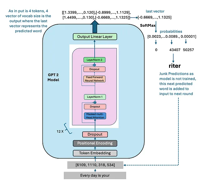
上面的图片还显示了我们未经训练的GPT模型预测的下一个单词。使用我们未经训练的模型，我们生成了5个新的标记（代码在这里 - Github）.

我们的输入文本是 - “每一天都是你的”，从未经训练的GPT 2模型中生成的下一个5个标记如下:

这是预期的，因为模型尚未经过训练。（无适配，无微调）

谢谢阅读！

感谢您的阅读！阅读完本文后，您将对GPT模型架构有更深的了解。如果您还没有阅读过GPT模型的演变，可以在这里阅读。接下来，我会发布关于训练这个LLM模型的文章。敬请关注。

代码库

请访问https://github.com/vipulkoti/BuildGPT2Model

参考资料【第一部分和第二部分】

[1] Radford, A., & Narasimhan, K. (2018). 通过生成式预训练改善语言理解。

[2] Radford, A., 吴, J., 孩子, R., 栾, D., 安莫得, D., & 苏茨凯弗, I. (2019). 语言模型是无监督的多任务学习者。

[3] Brown, T. B., Mann, B., Ryder, N., Subbiah, M., Kaplan, J., Dhariwal, P., Neelakantan, A., Shyam, P., Sastry, G., Askell, A., Agarwal, S., Herbert-Voss, A., Krueger, G., Henighan, T., Child, R., Ramesh, A., Ziegler, D. M., Wu, J., Winter, C., … Amodei, D. (2020). 语言模型是少样本学习器。arXiv。https://arxiv.org/abs/2005.14165

[4] OpenAI. (2023). GPT-4 技术报告. arXiv. https://arxiv.org/abs/2303.08774

[5] Ashish Vaswani, Noam Shazeer, Niki Parmar, Jakob Uszkoreit, Llion Jones, Aidan N Gomez, Łukasz Kaiser, 和 Illia Polosukhin. 注意力机制即为一切。NeurIPS, 2017.

[6] Raschka, S. (2023). 从头开始构建一个大型语言模型 [Https://www.manning.com/books/build-a-large-language-model-from-scratch]. Manning Publications Co. https://www.manning.com/books/build-a-large-language-model-from-scratch